3.0.1 The Nyquist Plot
As previously mentioned in Module 1, the Nyquist plot is one of the most common ways to quickly visualize and interpret raw EIS data. Based on the type of electrochemical system and its state, the shape of the Nyquist plot may differ. As temperature, state of charge, and health change, we can observe the differences in the Nyquist data. The interactive figure below shows the effect of state of charge on the Nyquist plot’s signature.
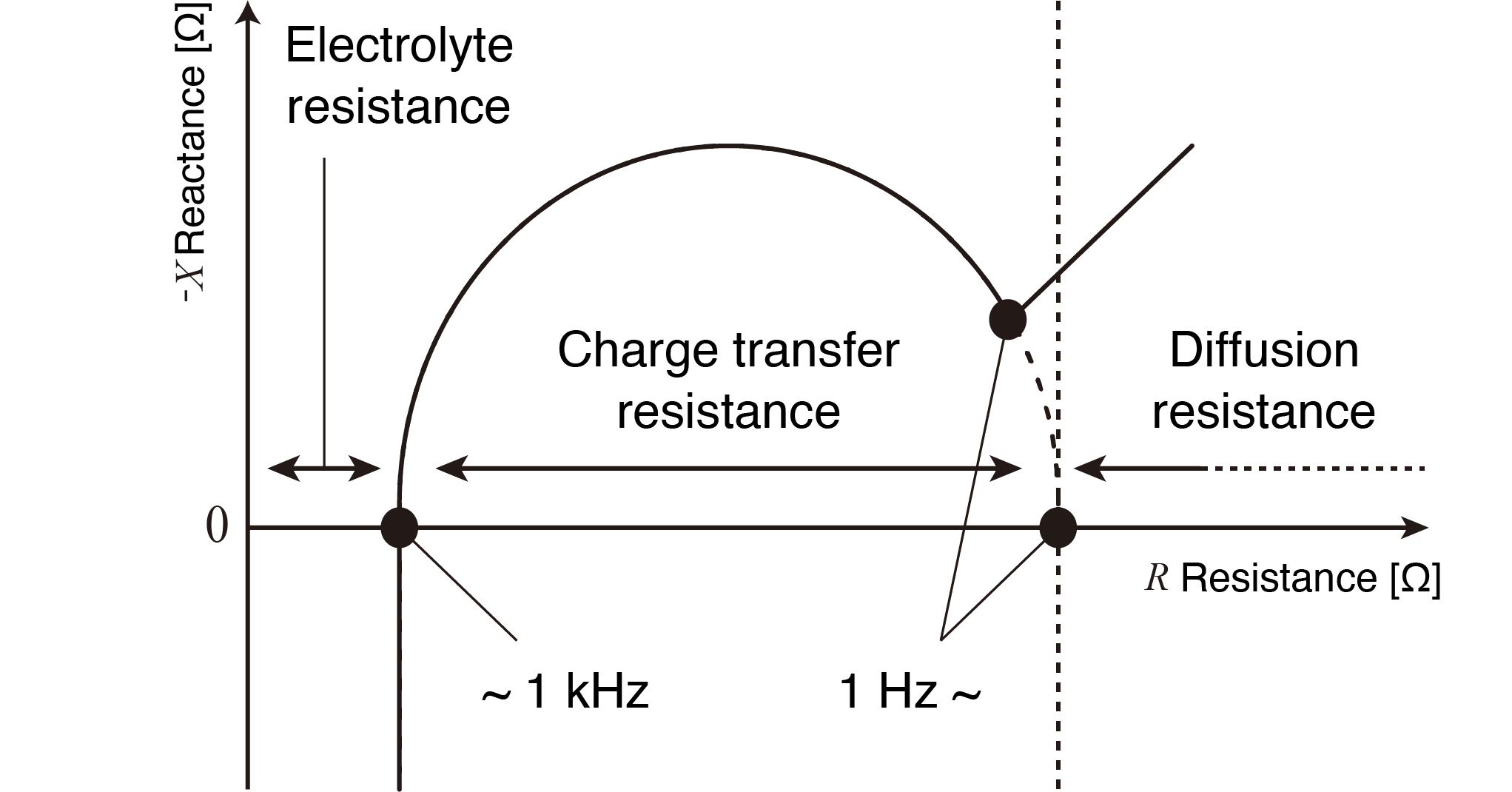
Basic visual analysis of the Nyquist plot can provide useful information towards building an accurate equivalent circuit model. Key areas of the figure for ECM development can be broken into the corresponding frequency regions. The high frequency region on the left side of the figure indicates if inductive effects are present, and can provide an initial estimate of the system’s bulk resistance at the x-intercept. The low frequency region on the right side exhibits slower processes such as diffusion. When an approximately 45-degree curve is present, this complex impedance can be modelled using a warburg resistor. The mid-frequency range can be harder to synthesize visually through the Nyquist, but it is equally important in the process of accurately modelling the system. The shape, size, and number of semi-circles in the mid-frequencies relate to the condition and number of interfacial processes present. Using this information, we can get a strong visual assessment of the system’s condition, and basis for beginning ECM analysis. Figure 2 acts as a guide for analyzing your Nyquist data.
3.0.2 Distribution of Relaxation Times
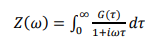
Distribution of relaxation times (DRT) helps to reveal overlapping processes that may not be visible in the Nyquist plot. By converting the frequency-dependent impedance data into the time-domain, distinct electrochemical processes can be analyzed using time constants. Time constants are a measure of a system’s response time to a given input. In this case, the time constants would represent the response times of electrochemical processes over varying timescales, such as charge transfer or diffusion. The expression in equation 1 computes the function of distributed time constants G(tau) given the measured impedance data Z(w).
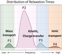
Prototypically, DRT data is visualized with the logarithmic time constants on the x-axis and distribution function on the y-axis. The number of peaks in the distribution function relates to the number of individual processes at specific time scales in the electrochemical cell. This is useful information for building the equivalent circuit model, as the number of DRT peaks translates to the number of RQ circuit elements required. As shown in the plot below, there are 4 peaks indicating that there should be 4 RQ pairs in the equivalent circuit model.
As the state of the system changes, the number and shape of the peaks may change as well. To extract accurate results from the DRT analysis, tuning the function’s regularization parameters is required. Regularization acts to simplify the system by smoothing noisy data to isolate the dominant peaks. There are two regularization parameters, alpha and the L1 ratio. The alpha parameter controls the strength of the regularization, and larger L1 values penalize heavily weighted model parameters. The interactive figure below allows you to control the ECM and regularization parameters to highlight how the DRT plot changes in response.
3.0.3 Example Equivalent Circuit Model Process
Using this information, and granted we have a valid EIS measurement, the equivalent circuit model can be built. This section will serve as a walkthrough of the full process for building an accurate ECM. This begins with your raw EIS data, including real impedance, imaginary impedance, and frequency data.
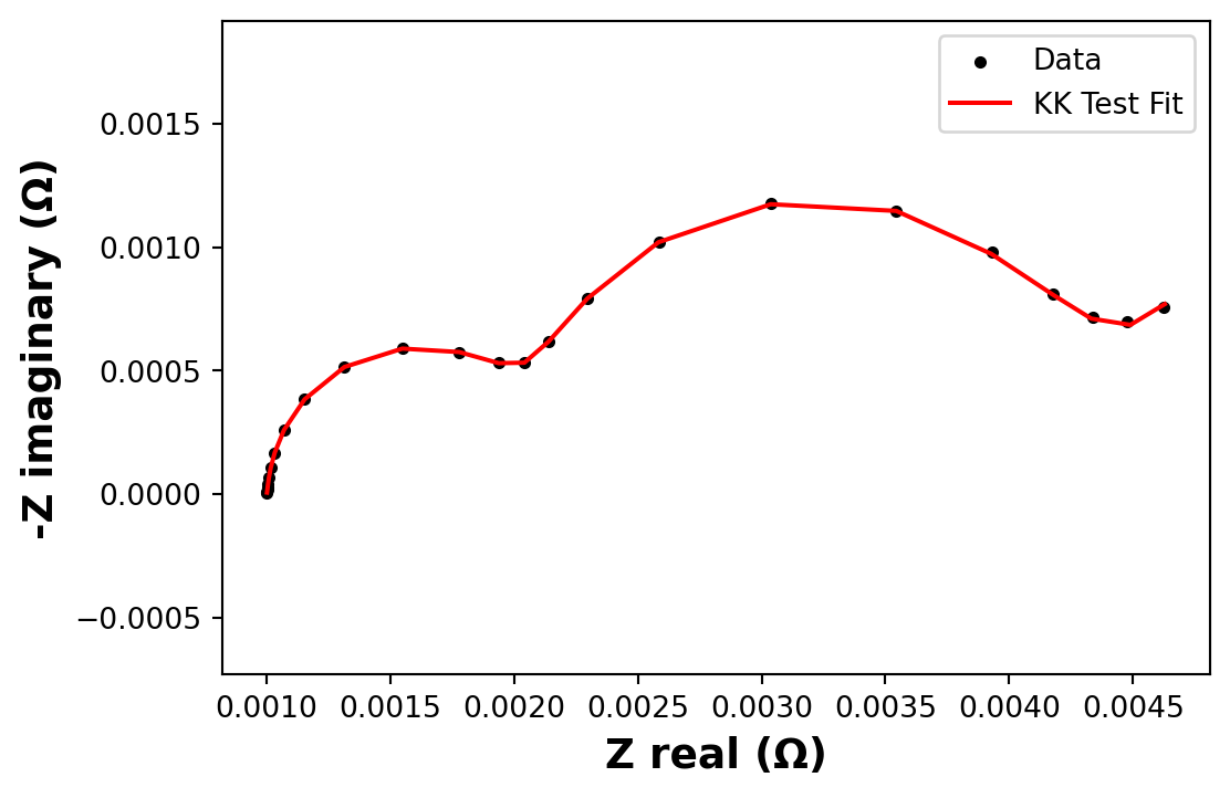
First, the EIS measurement data can be validated using the KK-test. The KK-test ensures the system is stable and linear by evaluating the residual error. Next, we can visualize the impedance columns and confirm a strong KK-test through the Nyquist plot. The overlaid KK-test model shows a good fit to the raw impedance data, indicating that we may proceed with this data. The Nyquist plot below provides an initial estimate of the electrolyte resistance at 5 ohms, and we can see that a warburg component should be added to the circuit based on the 45-degree slope in the low-frequency region. We can also determine that there are likely two RQ pairs based on the mid-frequency region, this can be confirmed with DRT analysis.
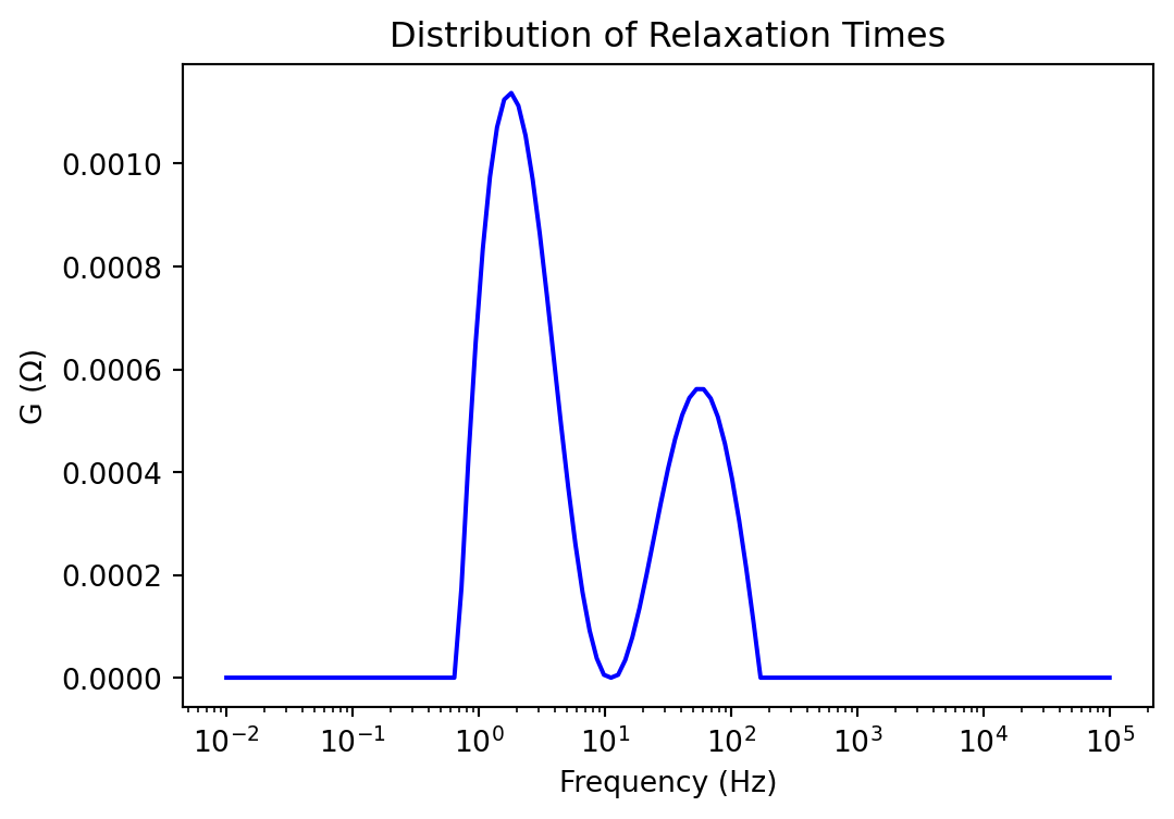
Next, we can solve the distribution of relaxation times to confirm the number of RQ pairs in the equivalent circuit model. The DRT plot below shows that there are 2 peaks, indicating that the circuit requires 2 RQ elements. If too many RQ are used in the ECM we risk overfitting the model and rendering the elements physically inaccurate.
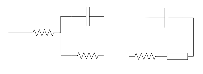
Based on our analysis, we can build the structure for an accurate equivalent circuit model. In summary, the Nyquist plot determined that a Warburg element should be added, and the DRT confirmed that there are 2 parallel resistor capacitor pairs. Figure 4 below shows a diagram of this system’s circuit.
Want to learn more? Speak with us today!
