When applying EIS to a system, it is crucial to correctly configure the input signal. This requires a careful balance between ensuring the signal’s amplitude is strong enough to be discerned from system noise, and not too large that the system becomes unstable or non-linear. This module will discuss the challenges of signal optimization, how to effectively set your EIS signal parameters, and how to validate your measurement. Following this procedure will ensure that the measurement requirements of linearity, causality, and stability are met.
2.0.0.1 System Stability
For an EIS measurement to be valid, the electrochemical system being measured must be operating in a steady state. This means that the current and voltage cannot be changing significantly over a short period of time. Whether or not a change in voltage or current is significant depends partially on the nature of the system itself and partially on the speed of the EIS measurement. If the measurement window for EIS is small, the relative change in voltage or current has less impact on the quality and validity of the EIS measurement.
2.0.0.2 Noise in the electrochemical system
When tuning the EIS signal, the noise of the electrochemical system is a factor that must be accounted for. Common sources of noise in an electrochemical system include broadband noise, interference from power sources, and noise at nearby unexcited frequencies and harmonics. If noise in the system is significant relative to the amplitude of the EIS signal being injected it will interfere with the EIS measurement. For an EIS measurement to be valid, the response of the system must be causal, meaning any perturbation must be predominantly a result of the EIS signal. Hence, it is important that the amplitude of the EIS signal is significantly larger than the noise in the system.
One common method of mitigating the effects of noise in the measurement is to average results over multiple data points to counter the randomness of noise. Another method is to increase the signal amplitude to overcome the noise threshold. The amplitude is tuned based on the signal-to-noise ratio, a high signal-to-noise ratio is necessary and should be valid across low and high frequencies. Since an acceptable signal-to-ratio will differ between systems, a source of feedback is required to properly tune the signal.
2.0.0.3 Non-linearity
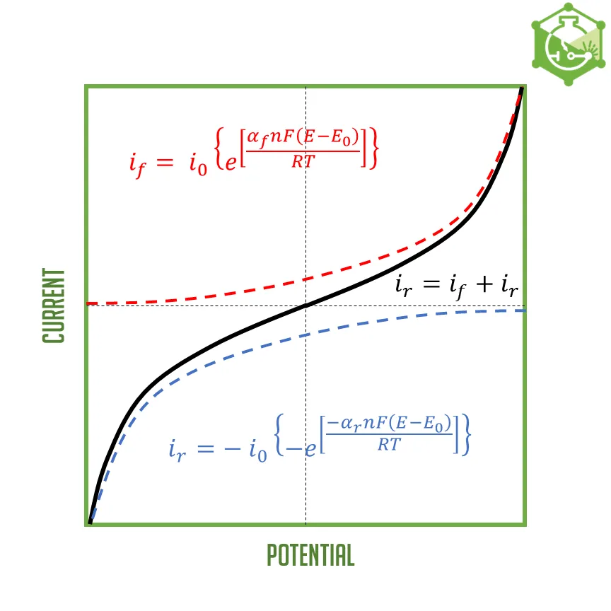
While overcoming system noise is required for EIS, the system must also remain linear where the change in current and voltage is directly proportional. Electrochemical systems are naturally non-linear as explained by the Butler-Volmer relationship between current density and cell voltage. The figure below shows that increasing current results in an exponential change in voltage and vice versa. To ensure linearity when performing EIS, it is best to operate in the pseudo-linear region by using sufficiently small perturbation where the change of current and voltage is approximately linear.
To achieve linearity the choice of running galvanostatic or potentiostatic EIS must also be considered. When dealing with low impedance systems potentiostatic control may result in large current flows inducing non-linearity following Ohm’s law. For this reason, galvanostatic EIS is recommended for lower impedance systems such as batteries.
2.0.0.4 Signal Validation
Now that the importance of linearity and the signal-to-noise ratio is established, a method of validating the measurement is required. Validation is imperative for effective signal optimization and ensuring all the required signal characteristics of linearity, causality, and stability are met. One method of validating data uses the Lissajous plot. The Lissajous plot of current and voltage will appear as a symmetrical ellipsis shape when the signal is optimal.
However, the most common method of validation uses the Kramers-Kronig relations. The Kramers Kronig relations are a set of mathematical equations that connect real and imaginary impedance. This allows for theoretical calculation of real and imaginary impedance that can then be compared against the measured system impedance for verification. The Kramers Kronig relations have been simplified to avoid the computation of complex integrals; and is denoted as the linear KK-test. The linear KK-test consists of an equivalent circuit model with N number of RC circuit elements that satisfies the KK relations [5]. The model is fit using linear equations and can be compared to the experimental data via Nyquist plot or residual error.
In practice we can see that the linear KK-test returns a plot of the Nyquist fit, the root mean square error (RMSE) of the fit, and the residual error. Using this information, it is possible to decipher if the measurement is strong enough based on whether the error of the KK test fit is below an outlined threshold and the residuals being random. If the residual errors are not random this may be an indication that the model is fitting to noise. The figure below is an example of a valid EIS measurement exhibiting strong accuracy metrics, model fit, and residual error.
Want to learn more? Speak to us today!
